Basic concepts in probability theory

Simple notions

What is probability?

Suppose we have a set \(\Omega\) and we have several events \(\omega\in\Omega\). If we randomly pick an event \(\omega\), we can ask: how frequently we will get an event satisfy certain criteria \(\Lambda\)? The probability to have event \(\lambda\in\Lambda\) is

\[ \lim_{N_t\to\infty}\frac{ N(\lambda\in\Lambda)}{N_t}; N_t\text{ is the number of trials.} \]

Probability of multiple variables

In statistical mechanics, usually we need to face probability descriptions of multiple variables. We will use a simple example to demonstrate the following concepts.

Suppose we have \(\Omega\) formed by integers with color red, green and blue.

\[ \Omega: \left\{Red: 1,34,7; Green: 12,5; Blue: 276, 19,18, 2331\right\} \]

In addition to the color, we can also categorize the integers by its parity, i.e. evenness or oddness.

We can use these two conditions, color and parity of the integers, to illustrate the following concepts.

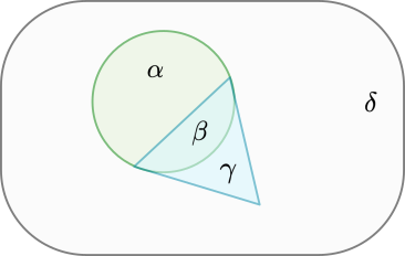
_images/probability.png — Fig. 4 The set \(\Omega\): The circled region, \(\alpha+\beta\), represent the red integers. The triangular region, \(\beta+\gamma\), represent the odd integers. The set \(\Omega\) is \(\alpha+\beta+\gamma+\delta\).

Joint probability

The joint probability ask what is the probability of two conditions to be true at the same time. For example, we can ask what is the probability that we have red odd integers? \(P(red,odd)=\frac{\beta}{\alpha+\beta+\gamma+\delta}=\frac{2}{9}\).

We have \(P(a,b)=P(b,a)\) in general.

The normalization condition for the joint probability is

\[ \sum_{a\in A}\sum_{b\in B}P(a,b)=1\xrightarrow{i.e.}\sum_{color}\sum_{parity}P(color,parity)=1\text{.} \]

Margin probability

The margin probability means we sum over all the possibilities of one condition. For example, we can ask what is the probability to have red integer in this case. We can derive that from the joint probability and sum over the even and odd cases with color red.

\[ P_A(a)=\sum_{b\in B}P(a,b)\xrightarrow{i.e.} P_{color}(Red)=\sum_{parity}P(Red,parity)=\frac{\alpha+\beta}{\alpha+\beta+\gamma+\delta}=\frac{3}{9}\text{.} \]

Conditional probability

Conditional probability of \(b\) given \(a\) is denoted as \(P(b|a)\). For example, we can ask what is the conditional probability of we pick a red integer given the integers are odd.

\[ P(red|odd)=\frac{\beta}{\beta+\gamma}=\frac{2}{5}\text{.} \]

\(P(a|b)\neq P(b|a)\) in general. For example

\[ P(odd|red)=\frac{\beta}{\alpha+\beta}=\frac{2}{3}\text{.} \]

Bayes’ theorem

\[\begin{split} P(a,b)=P(b,a)=P(b|a)P_A(a)=P(a|b)P_B(b)\\ \xrightarrow{i.e.} P(red,odd)=P(red|odd)P_{parity}(odd)=P(odd|red)P_{color}(red)\\ =\frac{\beta}{\beta+\gamma}\frac{\beta+\gamma}{\alpha+\beta+\gamma+\delta}=\frac{\beta}{\alpha+\beta}\frac{\alpha+\beta}{\alpha+\beta+\gamma+\delta}\text{.} \end{split}\]

Extended form of Bayes’ theorem when \(\Omega\) is divided into sub-regions \(\Omega_i\)

\[ P_B(b)=\sum_i P(b|\Omega_i)P(\Omega_i)\text{.} \]

We can pick \(\Omega_1=A\) and \(\Omega_2=\overline{A}\). Then we have

\[\begin{split} P(a|b)=\frac{P(b|a)P_A(a)}{P_B(b)}=\frac{P(b|a)P_A(a)}{P(b|a)P_A(a)+P(b|\overline{a})P_{\overline{A}}(\overline{a})}\\ \xrightarrow{i.e.} P(red|odd)=\frac{P(odd|red)P_{color}(red)}{P(odd|red)P_{color}(red)+P(odd|\text{not red})P_{color}(\text{not red})} \end{split}\]

Independent variables

If \(P(a,b)=P_A(a)P_B(b)\), we said \(a,b\) are independent variables.

This is because the conditional probability is \(P(a|b)=\frac{P(a,b)}{P_B(b)}\xrightarrow{independent}\frac{P_A(a)P_B(b)}{P_B(b)}=P_A(a)\) is independent of \(b\)!

Mean, variance and standard deviation

For a random variable \(a\) and the function \(F\) will map it to another random variable \(F(a)\).

Mean: \(\langle F\rangle \equiv \sum_a F(a) P_A(a)\).
n-th moment:\(\langle F^n\rangle \equiv \sum_a [F(a)]^n P_A(a)\).
variance \(\sigma^2=\langle (F-\langle F\rangle)^2\rangle=\sum_a \left(F(a)-\langle F\rangle\right)^2P_A(a)=\langle F^2\rangle-\langle F\rangle^2\)
correlation function between \(F,G\) is \(f_{FG}=\langle FG\rangle-\langle F\rangle \langle G\rangle\). That is, \( f_{FG}\equiv \sum_a\sum_b F(a)G(b)P(a,b)-\left(\sum_a F(a)P_A(a)\right)\left(\sum_bG(b)P_B(b)\right)\)

Gaussian integral

One-dimensional Gaussian integral.

\[ G_1=\int_{-\infty}^{\infty}e^{-ax^2}dx\text{.} \]

The trick is to square this expression, we found

\[ (G_1)^2=\int_{-\infty}^{\infty}\int_{-\infty}^{\infty}e^{-ax^2}e^{-ay^2}dxdy\text{.} \]

This integral is over a two-dimensional space; we can change the variables into polar coordinates \((r,\theta)\). The angular integral and the radial integral will become trivial.

\[ (G_1)^2=\int_{0}^{2\pi}\int_0^{\infty} e^{-ar^2}rdrd\theta=\frac{2\pi}{2}\int_0^\infty e^{-ar^2}2rdr=\frac{\pi}{a}\text{.} \]

Once this expression is known, we can simply generalize it into the case with a linear term

\[ G_1'=\int_{-\infty}^{\infty}e^{-ax^2+bx}dx\text{.} \]

The result will be left as an exercise.

Multidimensional Gaussian integral

The multidimensional Gaussian integral is

\[ G_N=\int_{-\infty}^{\infty}dx_1\int_{-\infty}^{\infty}dx_2...\int_{-\infty}^{\infty}dx_N \exp\left[-\frac{1}{2} x_iA_{ij}x_j+b_ix_i\right]=\sqrt{\frac{(2\pi)^n}{\text{det} A}} \left[-\frac{b_i(A)^{-1}_{ij}b_j}{2}\right]\text{.} \]

This expression can be derived by diagonalizing \(A\) and using the new basis to perform the independent one-dimensional integrals.

Stirling’s approximation

By definition

\[ N!=\int_0^{\infty}e^{-x}x^Ndx=\int_0^{\infty} e^{-x}e^{N\ln x} dx=\int_0^{\infty}e^{f(x)}dx\text{.} \]

This expression is exact. However, we want to have a good approximation of the \(N!\) which means we want to approximate the integral at the right-hand side when \(N\) is large.

We are going to introduce the idea of the steepest descent method (a.k.a. saddle point approximation) to derive Stirling’s approximation. We will do it first and then explain why this method makes sense. Let’s find the point \(x^{*}\) such that \(f'(x^*)=0\) and expand \(f(x)\) around \(x^{*}\).

We have

\[\begin{split} f(x)&= N\ln x-x=f(x^*)+f'(x^*)(x-x^*)+\frac{f''(x^*)}{2}(x-x^*)^2+...\\ f'(x)&=\frac{N}{x}-1\rightarrow x^{*}=N\\ f''(x)&=-\frac{N}{x^2}\rightarrow f''(x^{*})=-\frac{1}{N}\text{.} \end{split}\]

Next, we can ask: does it make sense to expand around \(x^*=N\)? To answer that we would like to know how the error looks like? The leading order error is proportional with \(f''(x^*)=-N^{-1}\). That means, when \(N\) is large, this error gets suppressed! The method of steepest descent is very general. However, one should analyze the error carefully. In this case, the form of \(f(x)\) works in our favor to suppress the leading order error! So we can approximate \(N!\) as

\[ N!\approx \int_0^{\infty}e^{f(N)-\frac{(x-N)^2}{2N}} dx=e^{N\ln N-N} \sqrt{2\pi N}\text{.} \]

This is Stirling’s approximation

\[ \ln N!=N\ln N-N+\frac{1}{2}\ln(2\pi N)\text{.} \]

One can insert \(N=10^{23}\) and see how important is each term. One can easily see the first two terms plays the dominant role in this expression.

What?

The method of steepest descent is a very powerful method to approximate integrals. Most of the time, we cannot evaluate integral exactly. Therefore, how to approximate the integral analytically is an important technique for analytic progress. We will refer our reader to [BO99] for detailed discussions.

Sets of independent random numbers

Suppose we have a vector \(\{F_1,F_2,...,F_N\}\) where \(F_j\) are independent random variables. In general, \(F_j\) is chosen from the probability distribution function \(P_j(F_j)\). (Mathematically, we allow \(P_j(F_j)\) to be arbitrary distribution functions. However, in physical settings, usually \(P_j(F_j)\) is a fixed function.) This is almost equivalent to our random walk problem. Let’s try to evaluate the sum of this vector.

\[ S_N=\sum_{j=1}^N F_j \]

The mean of \(S_N\) can be expressed easily

\[ \langle S_N\rangle=\sum_{j=1}^N \langle F_j\rangle \text{ (Here, we use the property that the mean is a linear operator).} \]

The variance of \(S_N\) is

\[\begin{split} \sigma_{S_N}=\langle S_N^2\rangle-\langle S_N\rangle^2=\sum_{j=1,k=1}^{N}\langle F_jF_k\rangle-\left(\sum_{j=1}^N F_j\right)\left(\sum_{k=1}^N F_k\right)\\ =\sum_{j=1}^{N}\sum_{k\neq j}^{N}\langle F_jF_k\rangle+\sum_{j=1}^{N}\sum_{k=j}^{N}\langle F_jF_k\rangle-\left(\sum_{j=1}^N F_j\right)\left(\sum_{k=1}^N F_k\right)\\ =\sum_{j=1}^{N}\sum_{k\neq j}^{N}\langle F_j\rangle\langle F_k\rangle+\sum_{j=1}^{N}\langle F_j^2\rangle-\left(\sum_{j=1}^N F_j\right)\left(\sum_{k=1}^N F_k\right)\\ =\sum_{j=1}^{N}\left[\langle F_j^2\rangle-\langle F_j\rangle^2\right]=\sum_{j=1}^{N}\sigma_j^2\text{.} \end{split}\]

In the third line of the equation, we use the condition that \(F_j\) are independent variables. That is, \(\langle F_jF_k\rangle=\langle F_j\rangle\langle F_k\rangle\).

The above expression is for a general distribution function \(P_j(F_j)\). If we are analyzing a specific physical system where \(P_j(F_j)=P(F)\), we can further simplify our result to have

\[\begin{split} \langle S_N\rangle= N \langle F\rangle\\ \sigma_{S_N}=N \left[\langle F^2\rangle -\langle F\rangle^2 \right]=N\sigma^2\text{.} \end{split}\]

The relative standard deviation is

\[ \frac{\sigma_{S_N}}{\langle S_N\rangle}=\frac{1}{\sqrt{N}}\frac{\sigma}{\langle F\rangle}\text{.} \]

This is the most crucial result of probability theory for statistical mechanics. What does it tell us?

When \(N\) is large (say \(N\approx 10^{23}\)), the fluctuation (estimated by \(\sigma_{S_N}\)) is barely noticeable compared with its mean value \(\langle F\rangle\) since this ratio goes as \(N^{-1/2}\).
The result is quite general; we only require the mean and the variance to be well defined. Not specific detail is required for \(P(F)\).
We can see that the problem actually gets simpler when \(N\to\infty\)!

Before we enter statistical mechanics

Why do we spend lectures talking about statistics?

The trivial reason: We need to those ideas for the future lectures.
The non-trivial reasons: it is related to two fundamental ideas of statistical mechanics.
1. \(N\approx 10^{23}\) could lead to regular behavior! The reason is simple; the relative deviations could be suppressed by large \(N\). Initially, it looks like large \(N\) gives us a formidable obstacle to understanding our system. However, now we realize that it could work in our favor to suppress the fluctuation.
2. The logical jump from microscopic detail description to statistical description: When \(N\) is large, the precise knowledge of microscopic components (e.g., molecules) is inessential to understand the system as a whole. We jump from the deterministic laws of physics from the microscopic physics to a pure probability description. This postulate is bold and is not obviously true. However, instead of proving this postulate, we will see the benefits of making this postulate in the following lectures.