Homework 2 — What Can a Basis Do? Flat Bands and Dirac Cones
Motivation
In Homework 1 and the lectures, we studied tight-binding models with a single site in each unit cell. In that case, after a Fourier transform, the Bloch Hamiltonian is essentially a scalar function .
In this homework we make the simplest non-trivial extension: put more than one site in a unit cell. The Bloch Hamiltonian then becomes a matrix,
and its eigenvectors acquire internal structure. We will see that this apparently small change allows qualitatively new phenomena:
and
The central question of this homework is therefore:
What new physics becomes possible when a unit cell contains more than one basis site?
Learning objectives
After completing this homework, you should be able to:
construct a Bloch Hamiltonian for a lattice with multiple sites per unit cell;
distinguish information contained in band energies from information contained in Bloch eigenvectors;
derive and interpret a simple flat band;
connect a flat band to destructive interference and compact localized states;
transfer a local interference mechanism from one lattice geometry to another;
derive the honeycomb-lattice band structure and identify its gapless points;
obtain a low-energy Dirac Hamiltonian by expanding around a band-touching point;
express a two-band Hamiltonian in the Pauli-matrix basis;
determine which perturbations shift a Dirac point and which perturbations open a gap.
Problem 1 — Can interference stop a particle from propagating?
1.1 The sawtooth chain: the simplest non-trivial flat band
Consider the periodic sawtooth chain shown in Figure 1. Each unit cell contains two sites, and . Let the hopping along the chain be , and let the hopping along the two diagonal bonds connecting each site to neighboring sites be .
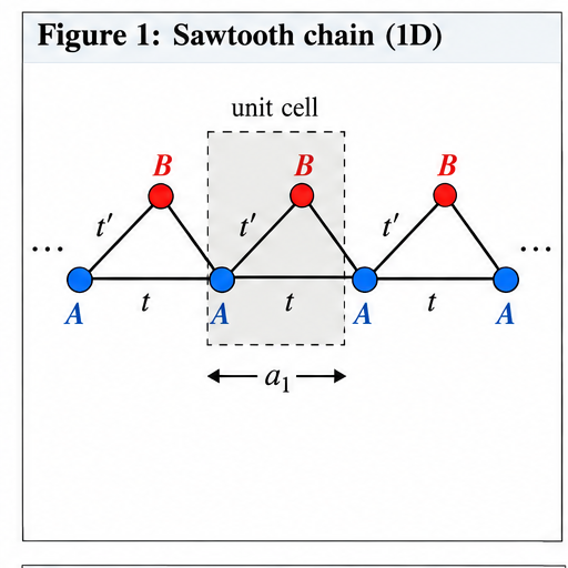
Figure 1:This is the sawtooth chain.
Take the tight-binding Hamiltonian to be
You may choose an equivalent unit-cell convention, but you must state it clearly and use it consistently.
(a) Bloch Hamiltonian
Introduce Fourier-transformed operators and write
Derive the Bloch Hamiltonian and obtain its two energy bands .
(b) Finding the flat-band condition
Determine the relation between and for which one of the two bands becomes completely dispersionless. State the corresponding flat-band energy.
Plot both bands over the first Brillouin zone for this special hopping ratio.
(c) The eigenvector matters
Find a Bloch eigenvector associated with the flat band.
The energy tells you that the band does not disperse, but the eigenvector contains information about why. Examine the relative amplitudes and phases on the two sublattices.
What feature of the eigenvector suggests destructive interference?
(d) Construct a compact localized state
Use the flat-band eigenvector as a clue to construct an exact real-space eigenstate whose amplitude is nonzero on only a finite number of sites.
Draw the nonzero amplitudes of your state, including their relative signs and magnitudes.
Act on the state with and verify explicitly that it is an eigenstate.
Identify the sites through which the particle could escape from the localized region.
Show that the hopping amplitudes into each such site cancel.
Explain in words why this cancellation prevents the state from propagating.
(e) Why does localization imply a flat band?
Translate your compact localized eigenstate by lattice vectors. Each translated state has the same energy.
Use this observation to explain physically why the corresponding band has no dispersion.
Your explanation should make clear the connection
1.2 Can you recognize the same mechanism without translational symmetry?
Now wrap the local geometry into the finite 12-site cluster shown in Figure 2. We will call this the Star-of-David cluster. Label the sites according to the figure and construct the nearest-neighbor tight-binding Hamiltonian
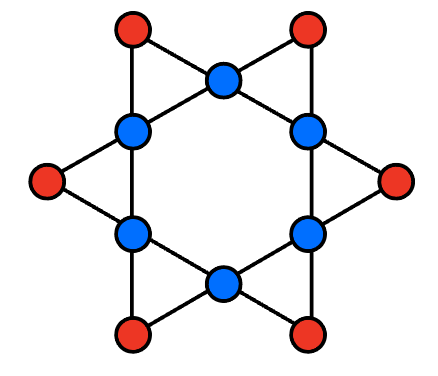
Figure 2:This is the 12 sites star of David cluster.
(a) Construct the finite Hamiltonian
Write the single-particle Hamiltonian matrix in the site basis
You may use a short numerical program to diagonalize it after constructing the matrix.
(b) Predict before diagonalizing
Before looking at the numerical eigenvectors, use what you learned from the sawtooth chain to propose a special eigenstate of this finite system.
Where should its amplitudes be nonzero? What relative signs should they have?
(c) Verify the interference mechanism
Verify directly that your proposed state is an eigenstate of the Hamiltonian.
Explain where destructive interference occurs and why the state remains localized even though the lattice contains allowed hopping paths out of its support.
(d) Conceptual question
There is no crystal momentum for this finite cluster. What, then, remains of the flat-band physics?
Explain which part of the mechanism is fundamentally local and which part requires translational symmetry.
1.3 From the sawtooth chain to the Kagome lattice
Consider the nearest-neighbor tight-binding model on the Kagome lattice shown in Figure 3. There are three sites, , , and , in each unit cell.
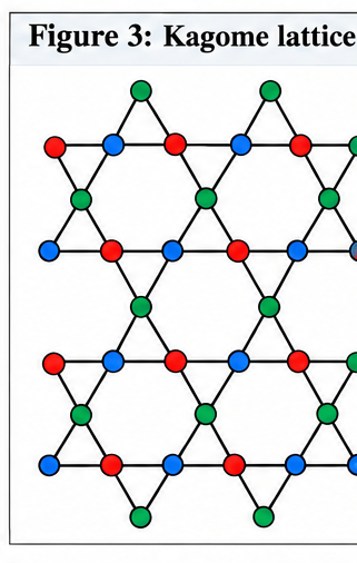
Figure 3:This is the partial picture of a Kagome lattice.
Take
(a) Bloch Hamiltonian
Choose primitive lattice vectors and and clearly specify the positions of the three basis sites.
Using
derive the Bloch Hamiltonian .
(b) Band structure
Diagonalize and obtain the three bands. Plot them along a suitable high-symmetry path in the first Brillouin zone.
Identify the flat band.
(c) Do not start from the algebra
Instead of treating the flat band merely as one root of a cubic characteristic equation, use the physical picture developed in Secs. 1.1 and 1.2.
Construct a localized eigenstate associated with a Kagome hexagon. Determine the relative amplitudes around the loop and show why hopping away from the loop cancels.
(d) Transfer of understanding
Compare the sawtooth-chain localized state, the Star-of-David state, and the Kagome localized state.
What is common to all three examples?
What aspects depend on lattice geometry, and what aspects do not?
Problem 2 — Can two bands meet without avoiding each other?
2.1 Nearest-neighbor honeycomb tight-binding model
Consider the honeycomb lattice shown in Figure 4. The lattice is not a Bravais lattice: each unit cell contains two inequivalent basis sites, and .
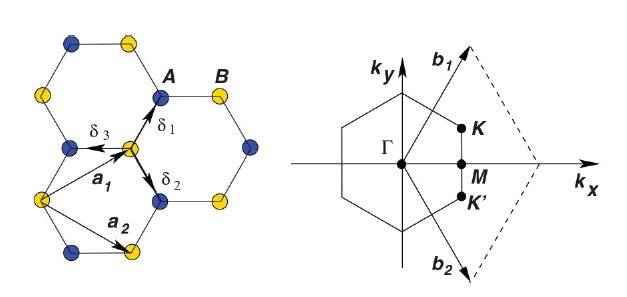
Figure 4:The left pannel is honeycomb lattice with . and . The right pannel is the Brillouin zone.
Let the three nearest-neighbor vectors connecting an site to its neighboring sites be , , and .
Consider
(a) Fourier transform
Derive the momentum-space Hamiltonian
Show that the off-diagonal element can be expressed through a structure factor of the form
up to your chosen convention.
(b) Band structure
Find the two energy bands .
Plot the band structure along a high-symmetry path such as
Use the right pannel of Figure 4 to identify the relevant high-symmetry points.
Locate the points where the two bands touch.
(c) Why can the bands touch?
At a generic momentum, two bands tend to avoid one another when they hybridize. Why does the honeycomb model nevertheless possess band-touching points?
Use the condition on to formulate your answer.
2.2 From a lattice model to the Dirac Hamiltonian
Choose one band-touching point, for example , and write
(a) Small-momentum expansion
Expand to leading nonvanishing order in .
(b) Pauli-matrix decomposition
Any Hermitian Hamiltonian can be written as
Identify the functions for the nearest-neighbor honeycomb model.
Show that near the gapless point the low-energy Hamiltonian takes the form of a two-dimensional massless Dirac Hamiltonian, up to convention-dependent signs and rotations of coordinates,
Determine the Fermi velocity in terms of the lattice parameters and hopping amplitude.
(c) What is the ``spin’’ in this Dirac Hamiltonian?
The Pauli matrices here do not need to represent the physical electron spin.
What two-dimensional degree of freedom do they act on in this problem? Explain why this is often called a pseudospin.
2.3 Is the Dirac cone an artifact of nearest-neighbor hopping?
A natural concern is that the Dirac Hamiltonian may simply be an accident of an overly simple tight-binding model. Let us perturb the model.
Add a real next-nearest-neighbor hopping between sites on the same sublattice, as illustrated in Figure 4 left pannel.:
(a) Modified Bloch Hamiltonian
Derive the new Bloch Hamiltonian and decompose it as
Which coefficient is changed by real, sublattice-symmetric next-nearest-neighbor hopping?
(b) Does the Dirac point survive?
Determine whether the two bands remain degenerate at and .
Expand again around a Dirac point. Does produce a mass gap, change the Dirac velocity, shift the energy of the Dirac point, or some combination of these?
Support your conclusion analytically and with a band-structure plot.
2.4 What actually gaps a Dirac point?
Now consider a staggered on-site potential
(a) Pauli-matrix interpretation
Show that this perturbation contributes a term proportional to
(b) Massive Dirac spectrum
Find the low-energy spectrum near and show that it has the form
with the appropriate for the model you are considering.
What is the size of the band gap?
(c) Compare the two perturbations
Explain why real next-nearest-neighbor hopping and a staggered sublattice potential have qualitatively different effects even though both modify the original nearest-neighbor model.
Use the Pauli-matrix decomposition to formulate a general rule:
Which terms can merely shift a Dirac point in energy, and which terms can gap it?
Synthesis — What did the basis vector buy us?
Answer the following questions concisely in your own words.
1. Energy versus eigenvector
Suppose you know only the band energies . What important physical information would you miss in the flat-band and Dirac examples studied here?
2. Two consequences of internal structure
Explain how having multiple basis sites in a unit cell enabled two apparently very different phenomena:
3. Local versus momentum-space thinking
The flat-band problem was most naturally understood through a real-space interference picture, whereas the Dirac problem was naturally understood through a momentum-space Hamiltonian.
Why are both descriptions useful? What does each reveal that the other may obscure?
Computational component
For this homework, your numerical work should be used to check and visualize analytical reasoning, not replace it.
Your submission should include at least the following student-generated plots:
sawtooth-chain bands at the flat-band hopping ratio;
Kagome bands along a stated high-symmetry path;
nearest-neighbor honeycomb bands along ;
honeycomb bands with nonzero real next-nearest-neighbor hopping, compared with the nearest-neighbor result.
Clearly label axes, hopping parameters, and momentum paths. Include enough code or pseudocode that your numerical calculation can be reproduced.
What you should take away
The purpose of this homework is not simply to diagonalize larger matrices. The important conceptual progression is
and from there two different pieces of physics emerge:
and
The eigenvalues are only part of an eigenvalue problem. Beginning with this homework, the structure of the eigenvectors will become increasingly important.